Image
- 1. Introduction
- 2. Image Menu
- 3. Toolbox
- 4. Image Area
- 5. "File" Window
- 6. "Colors" Window
- 7. 3-D Plot
- 8. "Cross-section" Window
1. Introduction
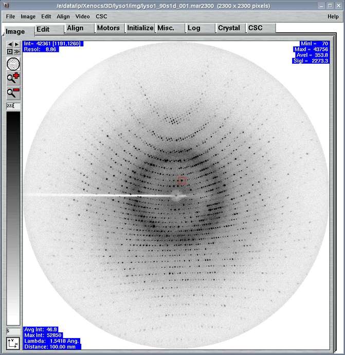
The "Image"-page can be accessed by selecting the corresponding tab in the main window or by pressing the "Ctrl+1"-key while the pointer is in the main window. This window is the area where to visually inspect images. The data display functions are very similar to those used by program marView with a couple of restrictions. You can:
- automatically display incoming images during data collection
- manually load images
- adjust color distributions of the image
- integrate areas of the image
- draw cross-sections of the image
- display resolution rings
- zoom in and zoom out
- print an image
The "Image"-page features several areas:
- a menu bar component called "Image" (see 2.)
- a tool box on left hand side of window (see 3.)
- an image display area with some information areas in upper left, upper right and lower left corners (see 4.)
During data collection, incoming images are loaded and displayed automatically, but only if the "Image"-page is up or if the Image menu-choice "Display image after scan" is selected. One should keep in mind, that image display puts load on the computer. During a data collection, it may not really be necessary to keep looking at images if everything proceeds nicely.
2. Image Menu
The Image menu pops up if the "Image" button in the menu bar is pressed or if "Alt+I" is pressed while the pointer is in the main window. The choices in the menu allow for opening additional windows or accessing special functions:
| Menu | Menu Choice | Shortcut | Description |
|---|---|---|---|
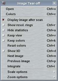
| Open | Ctrl+o | Pops up "File"-window |
| Colors | Ctrl+c | Pops up "Colors"-window | |
| Close | F1 | Takes away "Display"-window | |
| Show resolution rings | Ctrl+r | Toggle display of resolution rings | |
| Hide statistics | Ctrl+a | Toggle display of some image info in lower left corner | |
| Keep view | Ctrl+v | Keep same aspect of image and color scheme when loading new images. By default, image colors are recomputed and images are shown to fit in the window | |
| Keep colors | Ctrl+k | Keep same color scheme when loading new images | |
| Reset colors | Ctrl+t | Recomputes best color scheme for loaded image | |
| Show 3D | Ctrl+d | Toggle display of 3-D plots of zoomed areas (for zoom factors > 4) | |
| Next image | Ctrl+n | Load image with image number increased by 1 unit | |
| Previous image | Ctrl+p | Load image with image number decreased by 1 unit | |
| Integrate | Ctrl+i | Integrate the contents of the zoomed area and show results in upper right corner | |
| Zoom options | See "Zoom Options" submenu |
The choices in the "Zoom Options" submenu affect the way the image looks at zoom factors < 1.0. If one pixel on the monitor corresponds to more than 1 pixel (N pixels) in the image, image colors can be calculated in several ways. Please note, that "N'th" pixel mode is faster than others since it doesn't involve computation.
Table 3: The "Zoom Options" submenu
| Menu | Menu Choice | Description |
|---|---|---|
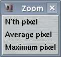
| N,th pixel | Use every N'th pixel to display colors and ignore others |
| Average pixels | Take average value out of N pixel to display colors | |
| Maximum pixels | Take maximum of N pixel to display colors |
3. Toolbox
The toolbox on the left hand side of the "Display"-window features the following functions:
| Toolbox | Symbol | Description |
|---|---|---|

| 
| Load previous image |

| Load next image | |

| Stop loading images (see next) | |

| Continuously load images by increasing image number | |

| Display entire image | |

| Zoom in | |

| Zoom out | |

| Upper limit for distributing grey scales | |

| Lower limit for distributing grey scales |
4 Image Area
4.2 Mouse Button Functions
Within the image area of the "Display"-window the mouse buttons have the following functions:
-
Left mouse button:
Press the left mouse and drag it to another position in the image. When the mouse button is released a window pops up showing the cross-section through the corresponding part of the image, i.e. a plot of pixel intensities starting at the position where the button has been pressed and ending at the position where the mouse has been released. In the image itself a red line will be drawn describing the trajectory. -
Middle mouse button:
If the area displayed in the window is magnfied (zoom factor >= 1, marked in the upper left corner of the display area), the coordinates of the mouse position and the intensity of the corresponding pixels are displayed in the lower left corner of the display area. Otherwise, the corresponding information is displayed in the upper left corner of the display area and, in addition, a box sized 50x50 pixels centered around that coordinate is integrated. The minimum, maximum and summed intensities are displayed in the upper right corner of the display area. A red box describing the contents of the box is drawn in the image area itself. -
Right mouse button:
If the area displayed in the window is magnfied (zoom factor >= 1, marked in the upper left corner of the display area), the displayed portion of the image is recentered around the coordinate of the mouse position. Thus, one can move around zoomed areas of the image. If zoom factors are smaller, than you can drag the right mouse button. A rectangle will be drawn in the image. If the button is released, the contents of the rectangle will be displayed. Depending of the size of the rectangle the corresponding zoom factor will be used. To increase and decrease the magnfication of the displayed part of the image, use the corresponding buttons with the magnification glass showing the "+" and "-"-sign.
4.3 Information Areas
In the corners of the image area of the "Display"-window certain information will be displayed, depending on previous actions:
-
Upper left corner:
When pressing the middle mouse button in the image area, the [x,y]-coordinate, intensity and resolution of the pixel under the pointer is displayed. -
Lower left corner:
Once an image has been loaded successfully, the most relevant information is displayed here: wavelength, distance, maximum intensity and average intensity. Display of this information may be removed by choosing "Hide statistics" in the Options menu -
Upper right corner:
When pressing the "Integrate"-button in the Options menu the following information is displayed: number of pixels in x and y, maximum, minimum, average, sum and standard deviation of pixel intensities, average background and mean intensity over background (all relative to the pixels displayed in the image area). The background is calculated from a histogram of intensities of a box of 50x50 pixels around the center of the zoomed area. Pixel values > 1000 are excluded from the histogram. Integration is possible only for zoom factors > 1.
5. "File" Window
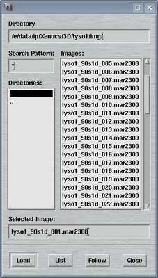
The "File"-window can be accessed by selecting the
corresponding choice in the "Windows"-menu
or by pressing the "Ctrl+f"-key while the pointer is in the display window.
This window is used to manually load images.
When the window pops up, the contents of the current working directory are listed in the file area of the window. By double-clicking a file, the corresponding file will be loaded. A single click will transfer the string of the selected file to the "Selected File:" area of the window and you will have to press the "Load"-button to actually load the image. By pressing the "List"-button, the directory is searched and files matching the "Search Pattern" are listed. By pressing the "Follow"-button a series of image files will be loaded. Image numbers will be continuously increased.
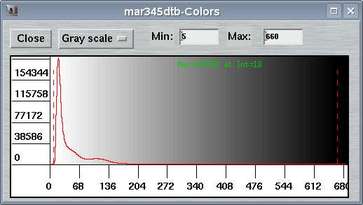
6. "Colors" Window
The "Colors"-window can be accessed by selecting the
corresponding choice in the "Windows"-menu
or by pressing the "Ctrl+c"-key while the pointer is in the display window.
This window is used to manipulate image colors.
The continuous red line in the plot shows the frequency of certain pixel values in the entire image, i.e. an intensity histogram. The maximum frequency is normally something like the average background or the "most probable" pixel value. In the histogram, two dashed bars mark the Min and Max values. To change Min or Max, enter values in the corresponding fields (and press RETURN!) or move the left or right bar using the left or right mouse button, respectively, and wait a moment until the image is rescaled accordingly.
When loading an image, the program automatically distributes grey scales in equidistant intensity bins between a minimum (Min) and maximum (Max) value. All pixel values > Max are drawn in black and all values < Min in white. Min usually is 0, but Max is calculated such that 99.998 % of all pixels in the image have intensities <= Max. The Max and Min can be entered in the upper part of the "Colors"-window or in the upper (Max) and lower text (Min) text field of the toolbox in the "Display"-window.
7. 3-D Plot
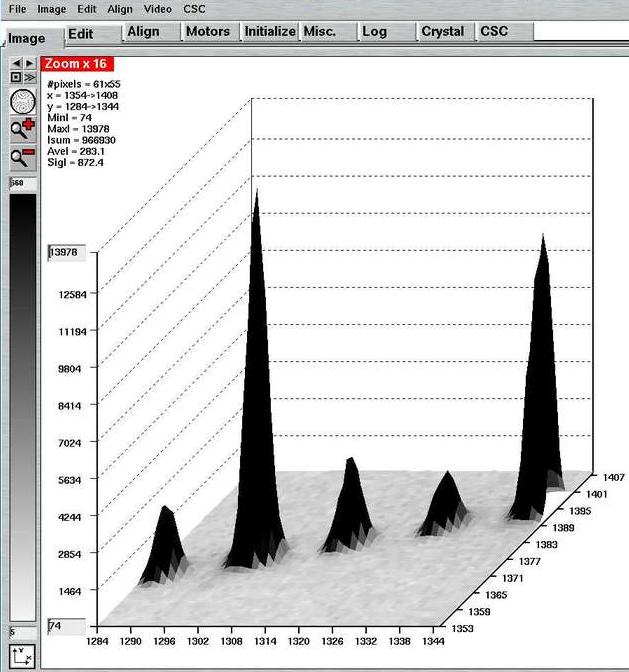
A 3-D representation of a portion of the image can be obtained
by selecting the "Turn ON 3-D plot"-choice in the
"Options"-menu
or by pressing the "Ctrl+d"-key while the pointer is in the display window.
This option works at zoom factors > 4 only. It dumps some statistics
of the displayed area in the upper left corner of the display area. The
aspect of the peak to be display may be altered by entering a minimum
or maximum threshold in the corresponding fields of the vertical axis.
As in the regular image area, the right mouse button may be used to
recenter the peak. This is a little bit of trial and error but once you
get used to it, it works. You may switch between 3-D and regular display
any time by pressing Ctrl+d.
8. "Cross-section" Window
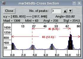
A cross-section through a portion of the image can be obtained
by dragging the left mouse button in the image area of the
"Display"-window. The window features the following
elements:
Table 1: The "Cross-section"-Window
| Element | Description |
|---|---|
| No. of peaks | Specifies the number of peaks between two dashed lines
in the plot area of the window. Use the arrow buttons on the right hand side of the fextfield to increment or decrement the value by 1. When pressed, the real space cell constant is calculated from the distance between the two dashed lines and the number of peaks. The result is displayed in the message area. |
| Message area | Shows the coordinates of the start and end of the line, the angle with the base line, maximum, minimum, average and standard deviation of the intensities along the drawn line. When changing the no. of peaks manually, the second line displays the derived cell constant. |
| Plot: vertical axis | Interpolated intensities |
| Plot: upper horizontal axis | Length of line in pixel units |
| Plot: lower horizontal axis | Length of line in mm units |
| Plot: left dashed line | Marks the beginning of a measured distance. This line can be moved using the left mouse button. |
| Plot: right dashed line | Marks the end of a measured distance. This line can be moved using the right mouse button. |
| Plot: horizontal red lines | Show the total length of the line in pixels (mm) and the distance between the dashed vertical lines. |
The pointer can be used to measure distances by setting the red dashed lines to the desired position along the drawn line. This is particularly useful if you want to measure cell constants. The program features a peak finding algorithm which tries to set the bars on top of the first and the last peak of the plot. Inbetween the peaks the program then looks for other peaks and tries to calculate the best inter-peak distances by assuming a harmonic oscillation. The no. of peaks calculated by the program is displayed in the "No. of peaks" textfield. Of course, this value can be modified. The derived cell constants do not take into account any particular setting or symmetry of the crystal but calculates cell constants assuming plain orthogonal axes.