2. GUI
- 2.1 Environment
- 2.2 Command Line Options
- 2.3 Main Pages
- 2.4 Plot Pages
- 2.5 Program Pages
2.1 Environment
The program makes use of different levels of environment variable settings. The program first looks for specific locations of the documentation directory tree (MARPRCDOCDIR), of the directory where to save the current session (MARPRCDATDIR) and of the directory where to look for specials files automar.defaults and cleanup.com (MARPRCDEFDIR).
If any one of the corresponding variables is not set, then the program looks for environment variables AUTOMARDOCDIR, AUTOMARDATDIR and AUTOMARDEFDIR, respectively.
If any one of these variables is not set, then the program steps one level further down and looks for environment variable AUTOMARDIR. The program now expects to find the documentation tree in subdirectory $AUTOMARDIR/doc and/or the session files and default files in $AUTOMARDIR/dat.
If the documentation directory doesn't exist, the documentation cannot be obtained by selecting the Contents-choice in the Help-menu. If the directory with the session files doesn't exist, the program will always use the working directory for saving session files.
The choice of which environment variables to use depends on local usage and personal preference. Some hints:
- Define MARPRCDOCDIR, MARPRCDATDIR and MARPRCDEFDIR if you are using automar, marFLM, marHKL, marXDS and other data procesing suites by marxperts simultaneously and if you want keep documentation in one place and also the session files.
- Only define MARPRCDOCDIR and MARPRCDEFDIR if you are using automar, marFLM, marHKL, marXDS and other data procesing suites by marxperts simultaneously and if you want keep documentation in one place but NOT the session files. By not defing MARPRCDATDIR, session files will be saved to the data processing (working) directory. This option is useful when working in multi-user environments where from the same account on the same host computer data sets from different crystals may be processed simultaneously (e.g. synchrotrons).
- Define AUTOMARDOCDIR, AUTOMARDATDIR and AUTOMARDEFDIR if you are using automar, marFLM, marHKL, marXDS and other data procesing suites by marxperts simultaneously and if you want keep documentation and the session files well separated
- Only define AUTOMARDOCDIR and AUTOMARDEFDIR but NOT AUTOMARDATDIR. See b) for details.
- Only define AUTOMARDIR if you want keep documentation and the session files separated from other program suites and if you prefer to use only one environment variable instead of 3.
- Don't define anything. The program will still work perfectly okay but you can't access the documentation. Otherwise, same behaviour as described in b).
The table below gives the environment variables used by program automar. The environment should best be defined within the shell startup scripts, i.e. files $HOME/.cshrc (C-shell) or $HOME/.tcshrc (TC-shell) or $HOME/.bashrc (Bourne-shell) using the usual nomenclature.
Environment variables used by automar
| Name | Description |
|---|---|
| MARPRCDOCDIR | Location of directory tree with documentation. |
| MARPRCDATDIR | Directory where to save current session parameters (automar.mix). |
| MARPRCDEFDIR | Directory where to find default session parameters (automar.defaults) and executable file cleanup.com |
| AUTOMARDOCDIR | Location of directory tree with documentation. Only used if MARPRCDOCDIR is not defined. |
| AUTOMARDATDIR | Directory where to save current session parameters (automar.mix). Only used if MARPRCDATDIR is not defined. |
| AUTOMARDEFDIR | Directory where to find default session parameters (automar.defaults) and executable file cleanup.com Only used if MARPRCDEFDIR is not defined. |
| AUTOMARDIR | Root directory for automar distribution. The program expects to find subdirectories $AUTOMARDIR/doc where all the documentation resides and $AUTOMARDIR/dat, the location of startup files and files that are stored automatically during program execution. Only used if other environment variables are not defined. |
2.2 Command Line Options
automar can be invoked in a terminal window plainly by typing automar. The program however understands the command line options given below.
Command line options for automar
| Name | Alternative | Description |
|---|---|---|
| -h | --help | Print usage summary |
| -v | --verbose | Increase printed output |
| -n | --nodisp | Disallows display of images. When working on 8-bit color displays, availability of colors may become a problem and the program may refuse to start due to lack of color cells. Since the image display is the actually color consuming part of automar "-n" leaves out the image display part and saves colors. |
| -g | --geometry | Specifies size and location of the main window
Use arguments: <width>x<height>+<x>+<y> Example: automar -g 900x600+320+200 |
| -c | --colors | No. of colors to use for image display.
Use arguments: <number> Example: automar -c 32 |
| DIR | (none) | Use DIR as working directory.
Example: automar /home/mar345/data |
| FILE | (none) | Image file to load.
Example: automar xtal_001.mar1200 |
2.3 Main Pages
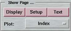
automar is logically divided into "pages". Some of them are dedicated to program input (see chapter: Program Pages) and others are for visual inspection, log file output, graphs, etc. Main pages can be chosen by pressing one of the buttons in the upper left corner of the interface, by selecting one of the choices in the Show Page menu in the menubar or by pressing keys F1, F2 or F3, respectively.
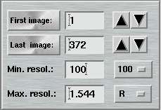
Also, in the main page you can select the single most often varied parameters common to all programs called by automar, in particular the image range for which to do the peak search and the integration ("First image" and "Last image") as well as the max. resolution limit. By pressing the First image-button and the Last image-button, the first and last image in the current directory are located and set into the corresponding fields, respectively.
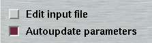
When running the programs from the GUI, you may want to have a look into the actual program command files before starting their execution. You may even edit them manually using an editor of your choice (File -> Preferences). To do so, check the "Edit input file"-box.
During the execution of a program, it is very handy to let automar automatically pick up refinement results and update the corresponding fields. Otherwise, you will have to do all the typing yourself. On the other hand, in certain situations, e.g. for mere testing purposes, you may want to disable automatic parameter update. Check the "Autoupdate Parameters"-box for this purpose. The parameters due to be autoupdated during indexing or postrefinement are:
- cell axes and angles
- spacegroup or lattice
- distance
- beam center
- mosaicity and divergence
- tilt, twist, turn of detector
- radial and tangential offset of detector
- crystal orientation angles
Note: The parameters that have been autoupdated without user interaction user will be drawn on a light pink background in order to draw your attention (see input parameters for marProcess). You may turn the autoupdating off by deselecting the toggle button. You may also manually edit the input file before actually starting a corresponding program.
While the Setup-area determines general crystal diffraction parameters
each single program step (peak search, indexing, etc.) can be fine tuned
by providing specific parameters. Please refer to
chapter 2.5 for details.
2.3.1 Text
The Text page features a large, scrollable text area. This is where
standard output of the programs go that are executed via automar.
The size of the fonts can be selected from the Preferences window
(selectable from menu File -> Preferences ...).
The Text page may be invoked by pressing the Text button
or by typing F3.
2.3.2 Setup
The Setup page is an input area for parameters that are common to more than one program called by the GUI. This is where you select the following parameters:
- working directory
- image data directory
- image name (root)
- image name extension
- crystal parameters (unit cell, spacegroup, etc)
- goniometer parameters (phi, delta-phi/image, distance, etc.)
- beam parameters (wavelength, divergence, polarisation)
- detector parameters (pixelsize, beam center, etc.)
2.3.2.1 Setup Directories and Names
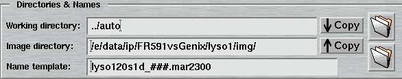
When selecting a working directory, it is convenient to click on the
![]() -icon on the right hand side of the "Working directory"-field.
A window pops up. You may move up and down through the directory tree
(always double-click).
Each time the directory is changed, the full path name is automatically
entered in the corresponding text field. This can save some typing and
also saves you from misspelling directory names.
-icon on the right hand side of the "Working directory"-field.
A window pops up. You may move up and down through the directory tree
(always double-click).
Each time the directory is changed, the full path name is automatically
entered in the corresponding text field. This can save some typing and
also saves you from misspelling directory names.
Hint: If a working directory doesn't exist, it may be created by entering the desired directory name and pressing return in the text field. A window will pop up that asks you to confirm or cancel the action.
When selecting an image directory, click on the
![]() -icon on the right hand side of the "Image directory"-field.
A window pops up. You may move up and down through the directory tree.
Each time the directory is changed, the full path name is automatically
entered in the corresponding text field. If you select a particular image
in the directory, there are additional benefits:
-icon on the right hand side of the "Image directory"-field.
A window pops up. You may move up and down through the directory tree.
Each time the directory is changed, the full path name is automatically
entered in the corresponding text field. If you select a particular image
in the directory, there are additional benefits:
- The image name is broken up automatically into 2 components: data directory and image name template. The program automatically tries to locate the image number fields - usually a 3 or 4-digit string - and replace it by the string '###' or '####', respectively. Since this procedure may not be 100% foolproof, it is always possible to adjust the name template manually.
- The program looks at the image header and presents the most relevant information: distance, phi, delta-phi, etc. You are asked if the corresponding fields in the "Setup"-page should be updated.
Close to the folder icons you can also see an arrow pointing downwards and one upwards. When pressing the "downwards" arrow, the directory name given in the "Working directory"-field is copied into the "Image directory"-field. When pressing the "upwards" arrow, the directory name given in the "Image directory"-field is copied into the "Working directory"-field. This, again, saves some typing.
2.3.2.2 Setup Crystal Parameters
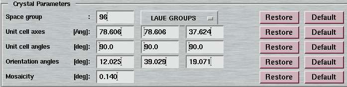
When working with program marIndex, the cell parameters need not be given as program input. Unit cell axes will basically be ignored when running the autoindexing, so the value entered doesn't matter at all. It is different with the spacegroup. If the spacegroup is unknown, a question mark ("?") will let the autoindexing make the best approximation of the lattice. What you will normally observe, though, is that suggested lattices tend to be the ones with less restraints for the cell angles, i.e. monoclinic rather than orthorhombic, etc.. By selecting a particular spacegroup, autoindexing will be forced to end with the setting angles to correspond to the desired space group, even if the quality of fit is not appropriate. Be aware that when running marIndex for the first time with an undefined spacegroup, the program will make its choice for the best lattice, and this choice will be taken automatically into the spacegroup field. When rerunning the program by just clicking the marIndex-button for the second time, the lattice is forced to the solution of the first run. If you don't want to impose restrictions on the lattice, you either have to deselect the "Autoupdate parameters"-check box or explicitely choose a "?" for the spacegroup in the Setup-page.
The field for the "Orientation angles" changes to "Missetting angles" if data integration step mosflm is selected. Note, that autoindexing yields unit cell orientation angles that describe the direction of axes {a, b, c} with respect to the goniometer coordinate system. These parameters are mostly used internally and are required for doing spot predictions with marPredict and strategy calculation with marStrategy but the user does not really need to be aware of them. In the case of mosflm, the setting angles are transformed into an orientation matrix that is stored in the file root_name.UMAT. Changes in the orientation matrix after postrefinement will be stored in the form of the missetting angles, which are small rotations required to readjust the orientation matrix to give the best fit of predicted to observed spots. In the case of denzo, the orientation angles are basically in the same form as used by the automar suite with one small difference: the sign of the second orientation angle is inverted! To stay in the mar convention, when writing out command files for denzo and when autoupdating postrefinement parameters the sign change is done automatically by the GUI so again the user does not have to be concerned about that.
Program marIndex comes up with a suggestion for the mosaic spread of the crystal. This value will be updated automatically. Postrefinement after integration is likely to yield a more accurate value.
2.3.2.3 Setup Goniometer Parameters
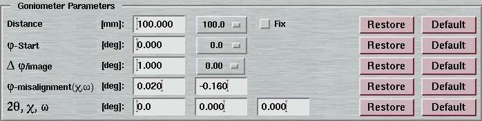
The goniometer parameters can be entered manually. It is more convenient to take them from image headers. See instructions in chapter "Setup Directories and Names" for loading image headers. Alternatively, choose option Read image header in the Options-menu of the menubar or press Ctrl+h to load the header of the image made up by components given in the "Image directory"-field, the "Image name root"-field, the "Image extension"-field and the the "First image"-field.
Note, that it is feasible to process data collected on a left-handed mar base (non-standard configuration with PHI rotating anti-clockwise) by setting the Chi-value to 180 deg.
2.3.2.4 Setup Beam Parameters
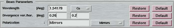
As described in the previous section, the wavelength should best be taken from the image header. Divergence and polarization are less critical values. If you really don't know what input to provide, go for the defaults.
There is a special implication, though, in the combination of wavelength "Cu" together with polarization "Mirrors": marIndex will test spots wether they are more likely due to K-beta radiation. This test will improve the refinement for the mosaicity.
2.3.2.5 Setup Detector Parameters
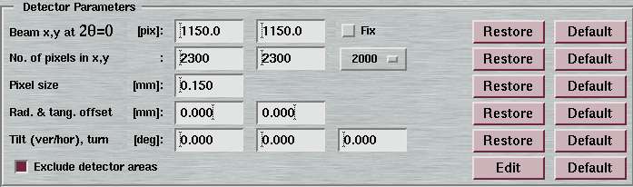
Program marIndex will refine the beam center and detector tilts, the radius of convergence being quite large. During postrefinement, more accurate parameters will become available. In particular, the radial and tangential offsets (for the image plate scanners) will be refined only by program ipmosflm. The latter ones should all be set to zero to start with.
The radial and tangential offsets apply only to spiral image plate scanners and not to CCD's. The offsets mark the deviation of the actual position of the scanner reading head at the start of the scan from the ideal position. The radial offset is the offset in radial direction (i.e. vertical) and may vary slightly from scan to scan, although the mar345-scanners should be fairly constant. The tangential offset is the offset in the horizontal direction and is supposed to be constant for all scans. It is not recommended to refine this parameter.
By checking the "Exclude detector areas"-box the entries in the "Excluded areas"-window will be used for running programs marPeaks, marPredict and data integration. Note, that not all choices avalaible in the window will be supported by all programs.
2.3.2.6 Exclude Detector Areas
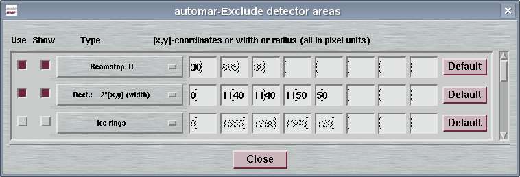
It is possible to systematically exclude unusable detector areas from peak search, spot prediction and integration. This is particularly useful for areas covered by the beamstop, by areas covered by obstacles (e.g. a cryo device) and also ice rings or other powder rings. The following choices are available for exclusion:
- beamstop: a circle around the beam center defined by a radius
- circle: a circle around a given pixel [x.y]
- ring: a concentric ring around the beam center defined by a min. and a max. radius
- rectangle: a box defined by coordinates of 2 opposite corners (plain rectangle) or by start and end coordinates of a line and an associated width (tilted rectangle)
- polygon: a quadrilateral defined by 4 coordinates
- ice rings: predefined rings at resolutions of 3.89 A, 3.67 A, 3.44 A, 2.67 A and 2.25 A
Note that all options are supported by all components of the automar suite of programs but not necessarily by ipmosflm or denzo. While denzo requires all input in mm units it turns out to be more convenient to operate with pixel units as shown in the image display area of this program. You must provide all coordinates and radii in pixel units. The middle mouse button can be used to obtain the required coordinates. To get visual feedback on the areas selected for inclusion, check the Show button.
2.3.3 Display
The Display page is the area where to visually inspect images. The data display functions are very similar to those used by program marView, but there are a couple of extensions. You can :
- manually load images or let them automatically load during program execution,
- manually load spot files or let them automatically load during program execution,
- add or delete spots from a spot file to be used for indexing,
- display spot predictions and/or integration boxes and profiles,
- print images,
- integrate areas of the image,
- draw cross-sections of the image,
- display resolution rings,
- zoom in and zoom out,
- determine the diffraction center with the aid of special tools.
Display toolbox

The Display-page features a small tool box shown at the top of the image area. The functions of the buttons are as follows:
Toolbox symbols
| Symbol | Description |
|---|---|

| Continue loading images going one step back in the history list until the beginning. |

| Load image going one step back in the history list. |

| Load image with image number incremented by 1 if at end of history list or load image one step ahead in the history list. |

| Continue loading images with image number incremented by 1 if at end of history list or continue loading images one step ahead in the history list. |

| Stop continuous image loading |

| Toggles automatical image loading during peak search, spot prediction and data integration |

| Save contents of display area into a graphics file (X-windows dump format = xwd). |

| Zoom out to display full image. Shortcut: Alt+0 |

| Incremental zoom in. Shortcut: Alt+p |

| Decremental zoom out. Shortcut: Alt+m |

| Display integration boxes and/or profiles. Enabled only when mosflm or DENZO spot file is loaded. |

| Display spot list from peak search or prediction |

| Edit spot list from peak search. Enabled only when peak search file is loaded. |

| Reload spot file |

| Pop up "Center Tool"-window. Shortcut: Alt+c |
2.3.3.1 Loading Images
To manually load an image, select "File -> Open Image ... " in the menubar (keyboard shortcut: Ctrl+o) and you get the "Open Image"-window. The program remembers the latest location where you loaded images from. When the window pops up, the contents of that directory are listed in the file area of the window. By double-clicking a file, the corresponding file will automatically be loaded. A single click will transfer the string of the selected file to the "Selected File:" area of the window and you will have to press the "Load"-button to actually load the image. By pressing the "List"-button, the directory is searched and files matching the "Search Pattern" are listed. By pressing the "List mar files"-button mar image files are listed, regardless of the search pattern. The program actually opens all files in the directory and determines automatically whether one file is a valid image file.
During execution of programs marPeaks, marPredict and marProcess/ipmosflm/denzo, currently processed images are being loaded automatically under 2 conditions:
- The "Display" page is selected.
- The "Autoload images"-button in the toolbox is selected.
One should also keep in mind, that image display can make the computer
work quite a lot. During an image integration run, it may not really
be necessary to keep looking at images if everything proceeds nicely,
so in that case one should probably switch over to the "Text"-page
or some other page, or (de-)select "Autoload" from time to time. "Autoload" from time to time.
2.3.3.2 Loading Spot Files
To manually load a spot file, select "File -> Open Spots ... " in the menubar (keyboard shortcut: Ctrl+p) and you get the "Open Spots"-window. The program remembers the latest location where you loaded spots from. When the window pops up, the contents of that directory are listed in the file area of the window. By double-clicking a file, the corresponding file will automatically be loaded. A single click will transfer the string of the selected file to the "Selected File:" area of the window and you will have to press the "Load"-button to actually load the spot file. By pressing the "List"-button, the directory is searched and files matching the "Search Pattern" are listed. By pressing the "List mar files"-button supported spot files are listed, regardless of the search pattern. The program actually opens all files in the directory and determines automatically wether one file is a valid spot file.
The program determines automatically which of the supported formats the spot file belongs to. There is no need to specify the spot file format in advance. Supported spot file formats are among others:
- .pks-files, i.e. peak search output by marPeaks
- .prd-files, i.e. spot prediction output by marPredict
- .i-files, i.e. integration output by marProcess
- .gen-files, i.e. integration output by ipmosflm
- .x-files, i.e. integration output by denzo
During execution of programs marPeaks, marPredict and
integration, currently
processed images and corresponding spot files are being loaded automatically
under the same conditions as given in section Loading Images.
2.3.3.3 Using Mouse Buttons
The 3 mouse buttons have all different functions.
- Left mouse button: press the left mouse and drag it to another position in the image. When the mouse button is released a window pops up showing the cross-section through the corresponding part of the image, i.e. a plot of pixel intensities starting at the position where the button has been pressed and ending at the position where the mouse has been released. In the image itself a red line will be drawn describing the trajectory.
- Middle mouse button: press the middle mouse. If the area displayed in the window is magnfied (zoom mode ≥ 1, marked in the upper left corner of the display area), the coordinates of the mouse position and the intensity of the corresponding pixels are displayed in the lower left corner of the display area. Otherwise, the corresponding information is displayed in the upper left corner of the display area and, in addition, a box sized 50x50 pixels centered around that coordinate is integrated. The min., max. and summed intensities are displayed in the upper right corner of the display area. A red box describing the contents of the box is drawn in the image area itself.
- Right mouse button: press the right mouse. If the area displayed in the window is magnfied (zoom mode ≥ 1, marked in the upper left corner of the display area), the displayed portion of the image is recentered around the coordinate of the mouse position. Thus, one can move around zoomed areas of the image. If zoom modes are smaller, than you can drag the right mouse button. A rectangle will be drawn in the image. If the button is released, the contents of the rectangle will be displayed. Depending of the size of the rectangle the corresponding magnification factor will be used. To increase and decrease the magnfication of the displayed part of the image, use the corresponding buttons with the magnification glass showing the "+" and "-"-sign in the upper part of the window.
2.3.3.4 Image Colors
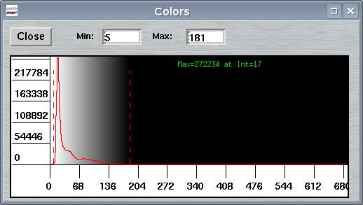
To manipulate image colors, select "Image Options -> Image Colors ... " in the menubar (keyboard shortcut: Ctrl+c) and you get the "Colors"-window. The continuous red line in the plot shows the frequency of certain pixel values in the entire image, i.e. an intensity histogram. The maximum frequency is normally something like the average background or the "most probable" pixel value. In the histogram, two dashed bars mark the Min and Max values. To change Min or Max, enter values in the corresponding fields (and press RETURN!) or move the left or right bar using the left or right mouse button, respectively, and wait a moment until the image is rescaled accordingly.
The program, when loading an image, automatically distributes 64 grey scales in equidistant intensity bins between a minimum (Min) and maximum (Max) value. All pixel values > Max are drawn in black and all values < Min in white. Min usually is 0, but Max is calculated such that 99.998 % of all pixels in the image have intensities <= Max. The Max and Min can be entered in the upper part of the "Colors"-window.
2.3.3.5 Image Options
Some tools related to image display can be accessed through the "Image Options"-menu in the menubar. The tools offered here are, in part, redundant. You can
- toggle display of resolution rings (shortcut: Ctrl+r),
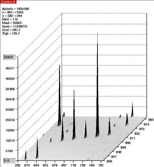
- toggle display of 3-D plots of zoomed areas (shortcut: Ctrl+d),
- toggle "Keep view", i.e. keep the same aspect of the image and color scheme when loading new images,
- toggle "Keep colors", i.e. keep the same color scheme when loading new images,
- change the zoom mode, i.e. display entire image (shortcut: Alt+0), zoom in (shortcut: Alt+p) or zoom out (shortcut: Alt+m),
- call the "Center Tool" (shortcut: Alt+c),
- integrate the contents of the zoomed area (shortcut: Alt+i).
The figure below gives a representation of the 3-D plot. This option works at zoom factors > 4 only. It dumps some statistics of the displayed area in the upper left corner of the display area. The aspect of the peak to be display may be altered by entering a minimum or maximum threshold in the corresponding fields of the vertical axis. As in the regular image area, the right mouse button may be used to recenter the peak. This is a little bit of trial and error but once you get used to it, it works. You may switch between 3-D and regular display any time by pressing Ctrl+d.
2.3.3.6 Center Tool
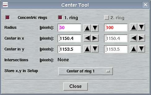
The "Center Tool"-window can be invoked from the "Image Options"-menu in the menubar or with shortcut Alt+c. It can be very useful to find the actual center of diffraction in an image. You may move to rings of variable size independent of each other within the displayed image, regardless of the zoom factor. By default, the center of the ring will be taken from the "Setup"-page. By default, both rings will be concentric but this feature can be deselected. The arrow buttons can be used to de- or increment ring radii or to relocate the center of the rings.
When looking at protein diffraction, the intersection of the lunes from different zones of reciprocal space determine the actual center of diffraction. You may therefore draw 2 circles along lunes that can be identified. The program calculates the intersection of the circles (if they do intersect, at all). The result - or the center of the first ring (magenta) or the center of the second ring (red) or the upper or the lower intersection of the rings - may be used as new beam center. The result may be directly transferred to the "Setup"-page.
2.3.3.7 Editing Spot Lists
If an editable spot file has been loaded, e.g. a spot file resulting from peak search by program marPeaks, the "Edit"-button in the toolbox of the "Display"-page is enabled. When pressing it you get additional buttons in the upper left corner of the display area:
"Edit Spots"-buttons
| Button | Name | Description |
|---|---|---|
| Add | Add new spots to the spot file by pressing the middle mouse button over the image. The added spots will be instantly displayed. Choose "Done" when finished. |
| Delete | Delete spots from spot list by pressing the middle mouse button over the cross marking an existing spot. There is a tolerance of some pixels for finding the actual spot. If the spot has been identified it is removed immediately. Choose "Done" when finished. | |
| More | Increase number of displayed spots. This reverses the action of "Fewer". Note, that you cannot get more than obtained by the run of program marPeaks (=100%). You must rerun marPeaks with other parameters to further increase the number of spots. | |
| Fewer | Decrease number of displayed spots. This is based on the I/sigma level in the marPeaks-type spot file. By pressing fewer, about 10% of the weakest spots will be removed. Removal is reversible by pressing "More". Choose "Done" when finished. After pressing "Done" you can not recover with "More". | |
| Done | Saves changes back to file and makes buttons disappear. |
2.3.3.8 Saving Graphics
The image currently displayed in the image area
can be saved to a file with all other features (integration boxes,
spot predictions, etc.) that are currently visible. The output format
is fixed (XWD = X Windows system window dump) and the file name is
the one of the loaded image with the additional extension ".xwd" added
to it. The {file_name}.xwd file can easily be converted to other
formats as PostScript, JPEG, GIF or whatever using graphics manipulation
programs like convert of the "Image Magick"-suite or
graphics visualization programs like xv, commonly available
on many Unix computers, in particular under Linux. To save the file,
press the  -button in the display toolbox.
2.4 Plot Pages
2.4.1 Index
The "Index"-page can be obtained by choosing the corresponding option in the upper left hand corner of the main window, by selecting the corresponding page in the "Show Page"-menu in the menubar or by pressing F4. It is used to graphically visualize the results from autoindexing. Technically, automar reads the log-file from program marIndex and extracts the relevant information. Results are presented in 3 areas:
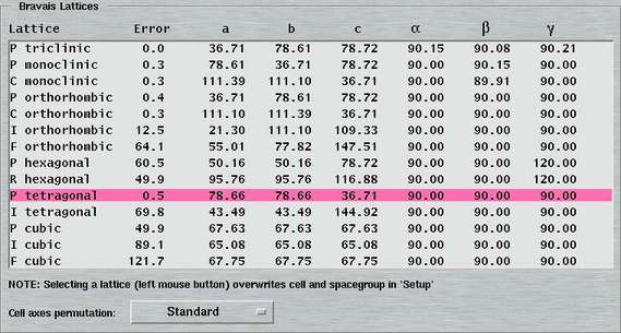
1.) Bravais lattices
List of 14 Bravais lattices with corresponding errors and cell parameters. The lower the error, the better the fit to the corresponding lattice type. You may use the left mouse button to transfer cell parameters of the selected lattice type directly to the corresponding fields (cell axes, angles and spacegroup) in the "Setup"-page. Note, that you MUST rerun marIndex when changing lattice selections, in order to obtain appropriate setting angles, etc.
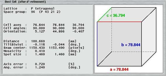
2.) Final results and cell
- Final refinement results for cell axes, distance, beam center, orientation angles, etc. Note, that the orientation angles are NOT to be confused with the "Missetting angles" in the "Setup"-page. The orientation given here is in marIndex notation. The resulting orientation matrix in ipmosflm notation is written out to the {file_name}.UMAT file. The mosaicity and spot sizes are refined on a weak data basis, only, so the values produced by marIndex should not be considered as being very accurate.
- Graphical representation of the final cell.
2.4.2 Strategy
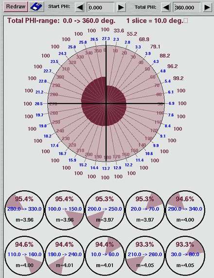
The "Strategy"-page can be obtained by choosing the corresponding option in the upper left hand corner of the main window, by selecting the corresponding page in the "Show Page"-menu in the menubar or by pressing F5. It is used to graphically visualize the results from strategy calculation. Technically, automar reads the log-file from program marStrategy and extracts the relevant information. It is normally a good idea, to simulate the entire Ewald sphere, especially since CPU-time for doing this should not be an issue any more. marStrategy then can find the best sections in the whole sphere for you. In the big circle plot, you will see first the completeness (red numbers outside the circle) increasing with increasing PHI ranges (black numbers inside the circle). The direction of rotation is given by the inner circle (magenta).
In the upper part of the display area you will find an input field for the "Starting PHI" and one for the "Total PHI". You may wish to play around with those values.
You can also save the plot to a graphics file by pressing the
button.
The resulting file is saved as Strategy.xwd in the current
working directory. See chapter
"Saving Graphics"
on comments about graphics files.
In the area underneath the big circle the top 8 best strategies are presented. The best strategy results from a scoring function and is a compromise between smallest PHI range to be covered, best completeness and best multiplicity, weighted in the order of appearance.
2.4.3 marPost
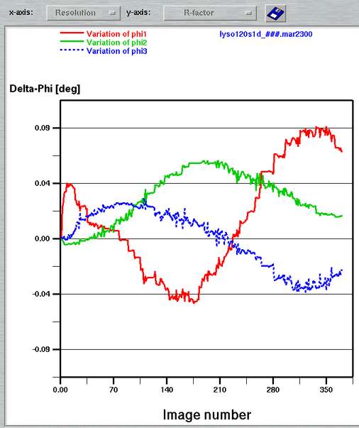
The "marPost"-page can be obtained by choosing the corresponding option in the upper left hand corner of the main window or by selecting the corresponding page in the "Show Page"-menu in the menubar. It is used to graphically visualize the refinement of orientation angles during integration. It plots the variations of the 3 orientation angles as a function of the image number. This plot may thus be used to quickly visualize any discontinuities of postrefinement and/or to unreveal crystal slippage or even hardware problems (e.g. sticking PHI-axis).
2.4.4 marScale
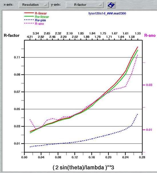
The "marScale"-page can be obtained by choosing the corresponding option in the upper left hand corner of the main window, by selecting the corresponding page in the "Show Page"-menu in the menubar or by pressing F6. It is used to graphically visualize the results from scaling and merging as produced by program marScale. Technically, automar reads the log-file from program marScale and extracts the relevant information. More than 20 plots are available for graphical visualization, the most relevant being the Rsym vs. resolution plot. Other plots can be selected from the menues in the upper part of the plot window.
You can also save the plot to a graphics file by pressing the
button.
The resulting file is saved as Resol:Rfac.xwd or alike in the current
working directory. See chapter
"Saving Graphics"
on comments about graphics formats.
Hint: With the left mouse button you can click into the plot. As a result, the y-axis-value of the closest item in the plot will be printed.
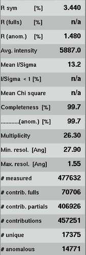
Besides different types of data plots, the "marScale"-page also provides an overview of the most important results of the scaling and merging step in the lower left area of the main window:
2.4.5 aimless
The "aimless"-page can be obtained by choosing the corresponding option in the upper left hand corner of the main window, by selecting the corresponding page in the "Show Page"-menu in the menubar or by pressing F7. It is used to graphically visualize the results from scaling and merging as produced by program aimless. It offers the same functions as the "marScale"-page as described in chapter above.
2.4.6 scalepack
The "scalepack"-page can be obtained by choosing the corresponding
option in the upper left hand corner of the main window, by selecting
the corresponding page in the "Show Page"-menu in the menubar
or by pressing F8. It is used to graphically visualize the
results from scaling and merging as produced by program scalepack.
It offers the same functions as the "marScale"-page as described
in chapter above.
2.5 Program Pages
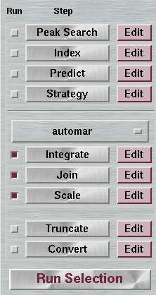
In the main window, on the left hand side, you will find an area where you can choose to run the desired program(s). Single program steps are run by pressing the corresponding button. The toggle buttons on the left hand side of the step buttons may be checked. By pressing the "Run Selection"-button all checked data processingsteps will be run in one go.
On the right hand side of the corresponding program name, you will find an "Edit"-button. When pressed, you can access areas to select program speficic options. In the majority of cases defaults might just work fine. On the other hand a program like ipmosflm offers dozens of keywords that have been introduced over a long period of time to take into account the large variety of diffraction phenomena observed on certain crystals. The automar-GUI offers only a reasonable selection of those options. In any case, fine-tuning is suggested only for those users who know what they are doing. Most settings are NOT subject to the trial-and-error approach.
A unique feature of the automar-GUI is the simultaneous support of 4 different data processing suites:
- marProcess + marScale
- ipmosflm + aimless
- denzo + scalepack
- xds + xscale
2.5.1 Peak Search
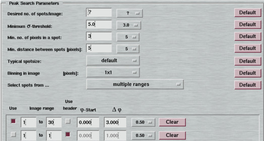
The "Peak Search"-page can be obtained by pressing the corresponding button on the right hand side of the "Peak Search"-button or by selecting the corresponding page in the "Edit Page"-menu in the menubar. This page offers a selection of the most frequently used variable parameters for program marPeaks. It is generally a good idea to use defaults and fine tune only where necessary.
The fields for the "Desired no. of spots/image" and the "Min. sigma-threshold" are mutually exclusive. Since an appropriate sigma-threshold is difficult to judge (mostly in between 10 and 30), it is easier to leave it at "Auto" and enter a value for the expected number of spots, instead, which can be guessed immediatley when looking at an image. Program marIndex however works best if there is a relatively large number of spots in the peak search file. The indexing algorithm itself eventually works with very few spots and will never use more than 200 spots but if a larger quantity of spots is presented it applies important additional criteria and uses only those spots that do contain the most valuable information.
By default, automar will do a peak search with the image number given in the "First image"-field in the main window, only. ending with the "Last image". If you wish to create spot lists from more than 1 consecutive oscillation range, you need to choose "Select spots from multiple ranges" and fill in the desired fields that will be visible. There are a few other choices which may or may not improve the quality of indexing.
For special cases, there is an option to set the expected average spot size in the diffraction pattern by making a choice on the menu for the "typical spotsize". Technically, this will modify some fine tune settings on the PEAK keyword for the program input. For diffraction pattern with large and fuzzy spots (e.g. neutron diffraction) it could make sense to choose "LARGE" or "HUGE" spots. Please refer to the man page of program marPeaks for further details.
Likewise, for diffraction patterns with very large spots there is an option to bin pixels in the image (e.g. 4x4). This obviously will increase the pixel size (done only internally) but can help to find suitable spots on diffraction patterns with few but very large spots.
2.5.2 Index
The "Index"-page can be obtained by pressing the corresponding button on the right hand side of the "Index"-button or by selecting the corresponding page in the "Edit Page"-menu in the menubar. This page is identical with the "Setup"-page obtained by pressing F2.
2.5.3 Predict
The "Predict"-page can be obtained by pressing the corresponding button on the right hand side of the "Predict"-button or by selecting the corresponding page in the "Edit Page"-menu in the menubar. This page is identical with the "Setup"-page obtained by pressing F2.
2.5.4 Strategy
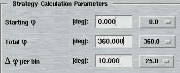
The "Strategy"-page can be obtained by pressing the corresponding button on the right hand side of the "Strategy"-button or by selecting the corresponding page in the "Edit Page"-menu in the menubar.
This page offers a selection of the most frequently used variable parameters for program marStrategy. It is generally a good idea to use defaults and fine tune only where necessary. It is recommended to calculate an entire Ewald-sphere up to the nominal resolution. The CPU-time should normally not be an issue.
It is recommended to use Delta-PHI ranges (for analysis) not smaller than 5 degrees. The accuracy of calculation will not really increase for smaller PHI ranges.
2.5.5 Integrate
The "Integrate"-page can be obtained by pressing the corresponding button on the right hand side of the "Integrate"-button or by selecting the corresponding page in the "Edit Page"-menu in the menubar. Depending on your choice of the data processing suite (automar, mosflm, denzo) the layout varies.
2.5.5.1 marProcess
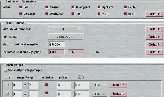
This page offers a selection of the most frequently used variable parameters for program marProcess. It is generally a good idea to use defaults and fine tune only where necessary. Besides the parameters given in this page, general parameters from the "Setup"-page will go in the parameter file for data integration as well. These are, namely, the crystal parameters (cell & spacegroup), the beam parameters, the goniometer settings and the geometrical parameters for the detector.
The spotsize is initially derived from the peak-search and will be used only as in initial estimate within marProcess. The seed-skewness method as implemented in marProcess automatically adjusts the spotsize in the course of the data processing. Hence, the value for spotsize given here does NOT have the same critical relevance as the corresponding parameters in program denzo. Only in pathological cases with many very close but not overlapping spots, one may have to fix the spotsize to a given value (in mm). Otherwise, fixing the spotsize is strongly discouraged, since it disables the application of the seed-skewness method.
Appendix 6.1.5.1 gives the analogy between input fields in automar and keywords in marProcess.
There might be data sets with interruptions in the middle of the data collection. This might be due to a problem with the X-ray source or discontinuities with the PHI-axis movement. It is still possible, to process such a data set within program marProcess in a single run by providing multiple image ranges. The benefit of doing this is that, presumably, most of the geometrical parameters don't vary within that data set. The overall data processing will become more homogeneous if all images are treated as belonging to one data set. For such cases, check "Use multiple image ranges" and specify the ones that you want to use. Unless the starting and Delta-PHI values are entered, those values will be derived from the ones given in the Setup window.
2.5.5.2 mosflm
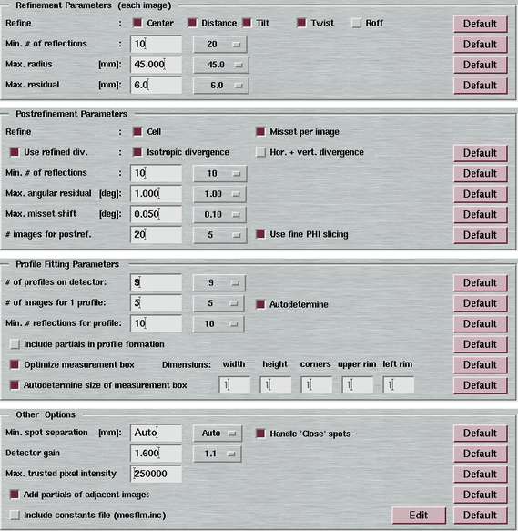
This page offers a selection of the most frequently used variable parameters for program ipmosflm. Appendix 6.1.5.2 gives the analogy between input fields in automar and keywords in ipmosflm.
2.5.5.3 denzo
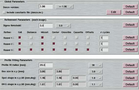
This page offers a selection of the most frequently used variable parameters for program denzo. Appendix 6.1.5.3 gives the analogy between input fields in automar and keywords in denzo.
Note, that program marIndex calculates an average spot size from the spot list as generated by program marPeaks. This spot size is used to automatically update the fields for Spot shape, BKG shape and Box size. By default, the BKG shape will be the Spot shape increased by 10% and the Box size will be calculated as 2*(Spot shape + 30%). As an additional help, it is useful to only edit the Spot shape parameters manually. When hitting the RETURN key while being in the text field, the program automatically updates the corresponding entry for BKG shape and Box size! When hitting RETURN while being in the BKG shape field only the Box size entry is modified.
2.5.5.4 XDS
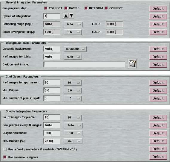
This page offers a selection of the most frequently used variable parameters for program XDS. Appendix 6.1.5.4 gives the analogy between input fields in automar and keywords in XDS.
Note, that program marIndex calculates an average spot size from the spot list as generated by program marPeaks. This spot size is used to automatically update the fields for Spot shape, BKG shape and Box size. By default, the BKG shape will
2.5.6 Join
2.5.6.1 marPost
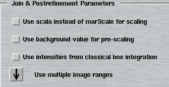
This page offers a selection of the most frequently used variable parameters for program marPost. Appendix 6.1.6 gives the analogy between input fields in automar and keywords in marPost.
It is rarely useful to use intensities from classical box integration, so this option should be left unchecked. For synchrotrons or other X-ray sources with strong fluctuations of X-ray dose from image to image a pre-scaling may be performed based on background values extracted from data integration. Another application would be fine-sliced data. But again, this option is usually not required.
2.5.6.2 sortmtz
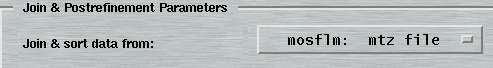
Program automar offers a common gateway for scaling data with program aimless of the CCP4-suite of programs, regardless if images have been processed with program marProcess, ipmosflm or denzo. During the "Join"-step the following needs to be done:
- If using data processed by marProcess (.i files) or denzo (.x files), data files need to be converted first into an mtz file. This is achieved by programs mar2mtz and rotaprep, respectively.
- The mtz files needs to be sorted using program sortmtz.
2.5.7 Scale
The "Scale"-page can be obtained by pressing the corresponding button on the right hand side of the "Scale"-button or by selecting the corresponding page in the "Edit Page"-menu in the menubar. Depending on your choice of the data processing suite (automar, mosflm, denzo) the layout varies.
Unless multiple data sets are specified explicitely within the corresponding parameter pages, the fields for the first and last image in the main window can be used to run the scaling program for a certain range of images. Likewise, the minimum and maximum resolution fields in the main window can be used to restrict the resolution of data merging and analysis.
2.5.7.1 marScale
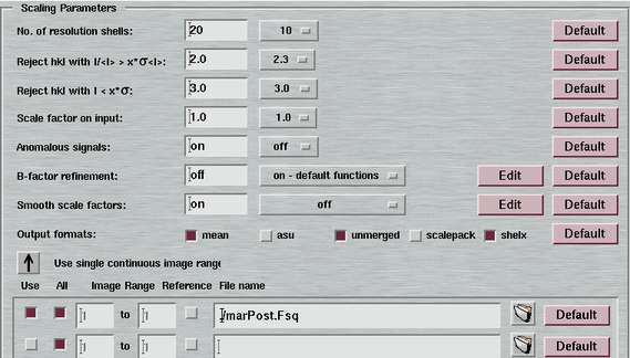
This page offers a selection of the most frequently used variable parameters for program marScale. It is generally a good idea to use defaults and fine tune only where necessary.
Appendix 6.1.7.1 gives the analogy between input fields in automar and keywords in marScale.
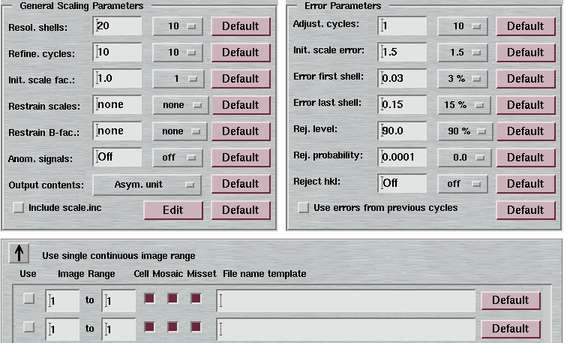
2.5.7.2 aimless
This page offers a selection of the most frequently used variable parameters for program aimless. It is generally a good idea to use defaults and fine tune only where necessary.
You may select to scale data processed not only by program ipmosflm but also by marProcess or denzo. This allows for quick comparison of results. For the latter options the data files from marProcess or denzo need to be converted first into an mtz-file and sorted. This achieved in the previous step ("Join").
Appendix 6.1.7.2 gives the analogy between input fields in automar and keywords in aimless.
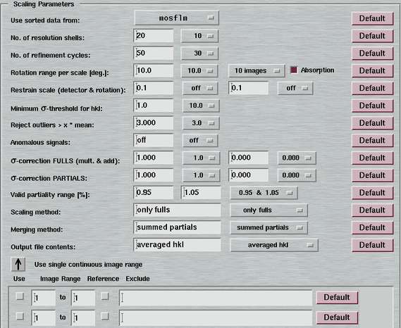
2.5.7.3 scalepack
This page offers a selection of the most frequently used variable parameters for program scalepack. It is generally a good idea to use defaults and fine tune only where necessary.
The scaling with scalepack relies on program scerror for determining the correct errors (sigmas) of the integrated reflections. Program scerror has been written and is being maintained by Dr. Victor Lamzin of the EMBL-outstation at DESY, Hamburg. This program is normally operated in a cyclical way. Program scerror analyzes the output of scalepack and provides an optimized error model. The final goal is to get all Chi-squares close to 1. Only then the sigmas may be considered to correspond to some physical truth. The recommended way of doing the scaling is to run a number of cycles, e.g. 10, of scalepack and scerror without rejecting any hkl. By then, scerror may already have converged in which case the adjustment cycles will automatically stop. So it wouldn't hurt to give a much larger number of cycles. Only then some more cycles may be run with rejections turned on - up to convergence. This approach works better if the number of resolution shells is not too small (press the Default button on Resol. shells for a reasonable value. Note, that when changing the number of resolution shells a previous run of scerror becomes invalid!
When "Use single continuous image range" is selected, the input files are generated from the current working directory, the image root name, the first and the last image number. Otherwise, multiple input files can be given.
Appendix 6.1.7.3 gives the analogy between input fields in automar and keywords in scalepack.
2.5.7.4 XSCALE
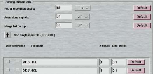
This page offers a selection of the most frequently used variable parameters for program XSCALE. It is generally a good idea to use defaults and fine tune only where necessary.
Appendix 6.1.7.4 gives the analogy between input fields in automar and keywords in XSCALE.
2.5.8 Truncate
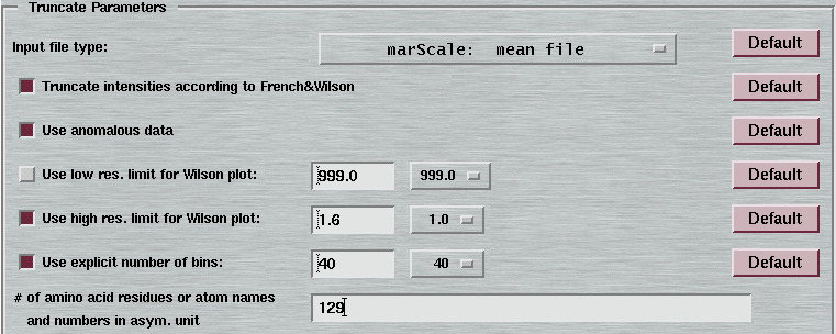
The "Truncate"-page can be obtained by pressing the corresponding button on the right hand side of the "Truncate"-button or by selecting the corresponding page in the "Show Page"-menu in the menubar.
This page offers a selection of the most frequently used variable parameters for program truncate. It is generally a good idea to use defaults and fine tune only where necessary.
The input file for program truncate needs to be an mtz-file. Program automar provides tools to directly convert the output of marScale and scalepack to mtz-files.
Appendix 6.1.8 gives the analogy between input fields in automar and keywords in truncate.
2.5.9 Convert
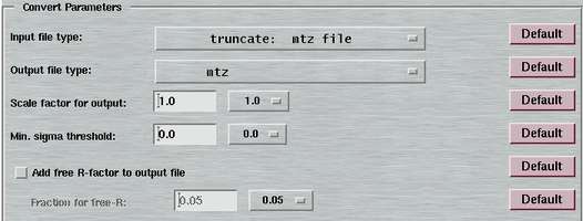
The "Convert"-page can be obtained by pressing the corresponding button on the right hand side of the "Convert"-button or by selecting the corresponding page in the "Edit Page"-menu in the menubar.
This page offers a selection of the most frequently used parameters for programs mtz2various, mar2mtz, scalepack2mtz, and scalepackcvt, respectively. It allows to produce a set of reflections used for free R-factor calculations. This option always go via programs from the CCP4-suite and - depending on input file type - intermediate files will automatically be created and deleted afterwards.
Appendix 6.1.9 gives the analogy between input fields in automar and keywords in mtz2various and others.